Interpolasi Kriging 2 Dimensi#
Penulis: Yudha Styawan
Install beberapa package berikut ini sebelum menjalankan notebook interpolasi.
pip install gstools pykrige rasterio
kita import package yang diperlukan
import numpy as np
import pandas as pd
from pykrige.ok import OrdinaryKriging
import matplotlib.pyplot as plt
from sklearn.metrics import r2_score
from rasterio.transform import from_origin
import rasterio
from scipy.spatial import cKDTree
import gstools
selanjutnya adalah membuka data. Data yang digunakan secara default berupa tab delimiter. Contoh datanya berikut ini:
lon	lat	val
116.36	2.015	-0.001226
116.36	2.114	-0.002219
116.36	2.214	-0.003445
116.36	2.313	-0.00492
116.36	2.412	-0.006635
...
df = pd.read_csv("test.dat", sep="\t"); df
| lon | lat | val | |
|---|---|---|---|
| 0 | 116.36 | 2.015 | -0.001226 |
| 1 | 116.36 | 2.114 | -0.002219 |
| 2 | 116.36 | 2.214 | -0.003445 |
| 3 | 116.36 | 2.313 | -0.004920 |
| 4 | 116.36 | 2.412 | -0.006635 |
| ... | ... | ... | ... |
| 886 | 118.96 | 4.798 | -0.009103 |
| 887 | 118.96 | 4.897 | -0.007640 |
| 888 | 118.96 | 4.996 | -0.006187 |
| 889 | 118.96 | 5.096 | -0.004835 |
| 890 | 118.96 | 5.195 | -0.003631 |
891 rows × 3 columns
ini opsional saja, untuk data coulomb stress, kita akan clip hingga di kisaran -1 hingga 1.
jika tidak ingin melakukan clip data, fungsinya data diubah sebagai berikut:
def fwd(val): return val
def fwd(val):
    return np.clip(val, -1, 1)
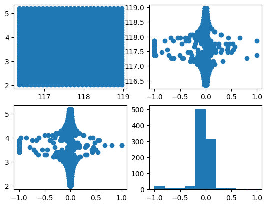
sebelum melakukan kriging, terlebih dahulu cek sebaran datanya, apakah data tersebut memiliki tren atau tidak.
fig, axs = plt.subplots(2,2)
axs[0,0].scatter(df.lon, df.lat)
axs[0,1].scatter(fwd(df.val), df.lon)
axs[1,0].scatter(fwd(df.val), df.lat)
axs[1,1].hist(fwd(df.val))
plt.show()
print(fwd(df.val))
0     -0.001226
1     -0.002219
2     -0.003445
3     -0.004920
4     -0.006635
         ...
886   -0.009103
887   -0.007640
888   -0.006187
889   -0.004835
890   -0.003631
Name: val, Length: 891, dtype: float64
kita masukkan datanya ke dalam dictionary untuk mempermudah penggunaan variabel kedepannya.
# Data scatter spasial: (x, y, T)
data = {
    "x": df.lon.to_numpy(),
    "y": df.lat.to_numpy(),
    "T": fwd(df.val.to_numpy()),
}
cek terlebih dahulu apakah variogram yang dipilih sudah cocok atau tidak. Ubah bagian ini untuk coba-coba:
model = gstools.Exponential(dim=2)
model = gstools.Gaussian(dim=2)
model = gstools.Spherical(dim=2)
model = gstools.Exponential(dim=2)
bin_center, gamma = gstools.vario_estimate(
    pos=[data["x"], data["y"]],
    field=data["T"],
    # estimator="cressie",
)
model.fit_variogram(bin_center, gamma)

# output
ax = model.plot(x_max=max(bin_center))
ax.scatter(bin_center, gamma)
plt.show()
print(model)
/Users/yudhastyawan/miniconda3-arm/envs/pydask/lib/python3.10/site-packages/gstools/covmodel/plot.py:122: UserWarning: FigureCanvasAgg is non-interactive, and thus cannot be shown
  fig.show()
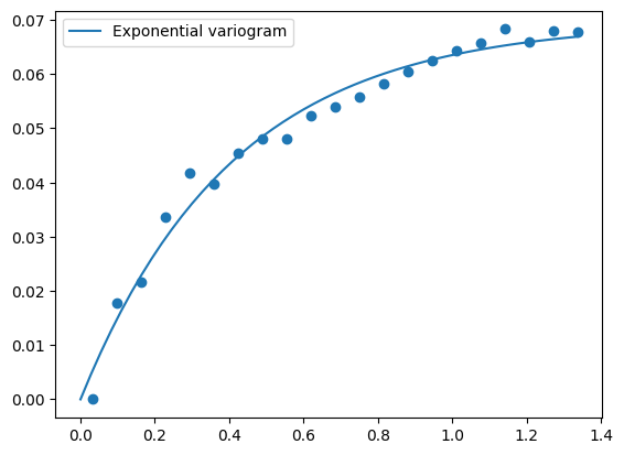
Exponential(dim=2, var=0.0696, len_scale=0.41, nugget=4.17e-18)
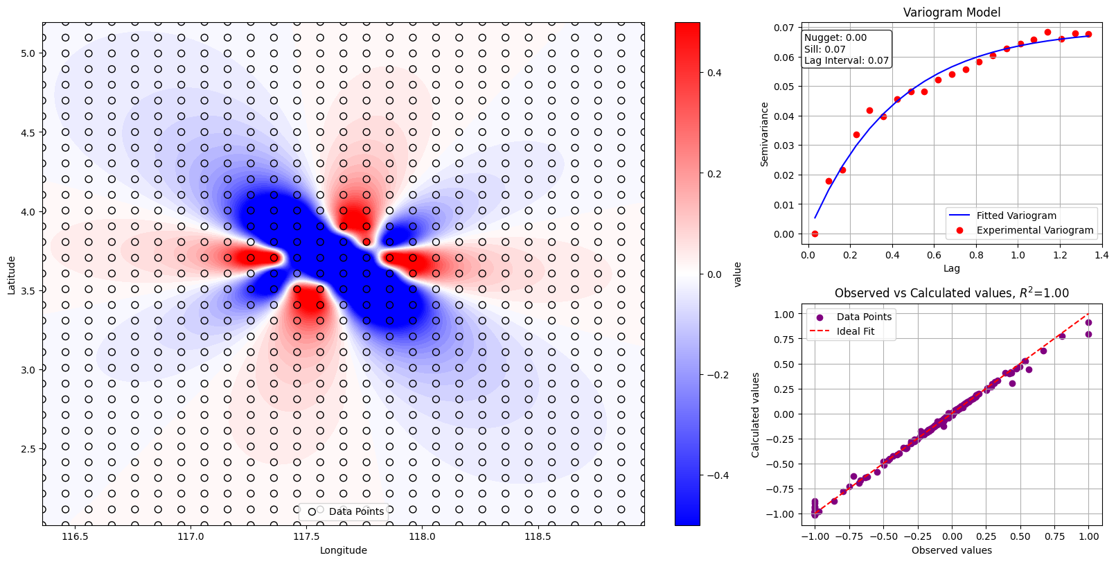
waktunya menjalankan kriging dan interpolasi.
# Membuat grid teratur untuk interpolasi
x_grid = np.linspace(min(data["x"]), max(data["x"]), 200)
y_grid = np.linspace(min(data["y"]), max(data["y"]), 200)
x_mesh, y_mesh = np.meshgrid(x_grid, y_grid)

# Melakukan kriging menggunakan Ordinary Kriging
ok = OrdinaryKriging(
    data["x"], data["y"], data["T"],
    variogram_model=model, # Anda bisa mengganti model variogram (e.g., "spherical", "exponential")
    verbose=True,
    enable_plotting=False,
)
z_mesh, ss = ok.execute("grid", x_grid, y_grid)
Adjusting data for anisotropy...
Initializing variogram model...
Coordinates type: 'euclidean'

Using Custom Variogram Model
Calculating statistics on variogram model fit...
Executing Ordinary Kriging...
# Membuat plot kontur
vmin = -0.5
vmax = 0.5

# Membuat plot kontur
fig = plt.figure(layout="constrained", figsize=(16, 8))
gs = fig.add_gridspec(2,3)
ax1 = fig.add_subplot(gs[0:2,0:2])
contour = ax1.contourf(x_mesh, y_mesh, z_mesh, cmap="bwr", levels=80, vmin=vmin, vmax=vmax)
scatt = ax1.scatter(data["x"], data["y"], c=data["T"], cmap="bwr", edgecolor="k", s=50, label="Data Points", vmin=vmin, vmax=vmax)
cbar = plt.colorbar(scatt, label="value")
plt.xlabel("Longitude")
plt.ylabel("Latitude")
plt.legend()

# Menampilkan model variogram
lags = bin_center
semivariance_obs = gamma
fitted_semivariance = model.variogram(bin_center)
nugget = model.nugget
sill = model.sill
lag_interval = lags[1] - lags[0] if len(lags) > 1 else 0

ax2 = fig.add_subplot(gs[0,2])
ax2.plot(lags, fitted_semivariance, label="Fitted Variogram", color="blue")
ax2.scatter(lags, semivariance_obs, label="Experimental Variogram", color="red")
plt.xlabel("Lag")
plt.ylabel("Semivariance")
plt.title("Variogram Model")
plt.legend()
plt.grid()
plt.annotate(f"Nugget: {nugget:.2f}\nSill: {sill:.2f}\nLag Interval: {lag_interval:.2f}",
            xy=(0.01, 0.95), xycoords="axes fraction", verticalalignment="top",
            bbox=dict(boxstyle="round", facecolor="white", alpha=0.8))

# Plot korelasi antara data observasi dan data kalkulasi
z_observed = data["T"]
calculated_points = np.column_stack((x_mesh.ravel(), y_mesh.ravel()))
kdtree = cKDTree(calculated_points)
nearest_indices = kdtree.query(np.column_stack((data["x"], data["y"])))[1]
z_calculated = z_mesh.ravel()[nearest_indices]

# Menghitung R-squared
r_squared = r2_score(z_observed, z_calculated)
print(f"R-squared: {r_squared}")

ax3 = fig.add_subplot(gs[1,2])
ax3.scatter(z_observed, z_calculated, color="purple", label="Data Points")
ax3.plot([min(z_observed), max(z_observed)], [min(z_observed), max(z_observed)], color="red", linestyle="--", label="Ideal Fit")
plt.xlabel("Observed values")
plt.ylabel("Calculated values")
plt.title(f"Observed vs Calculated values, $R^2$={r_squared:.2f}")
plt.legend()
plt.grid()

plt.savefig(f"test_interp_result.png", dpi=330)

# Menyimpan hasil interpolasi dalam bentuk raster .tif
transform = from_origin(x_grid[0], y_grid[-1], x_grid[1] - x_grid[0], y_grid[1] - y_grid[0])
with rasterio.open(
    f"test_kriging_result.tif",
    "w",
    driver="GTiff",
    height=z_mesh.shape[0],
    width=z_mesh.shape[1],
    count=1,
    dtype=z_mesh.dtype,
    crs="EPSG:4326",
    transform=transform,
) as dst:
    dst.write(z_mesh[::-1,:], 1)

plt.show()
R-squared: 0.9955079038457918
selesai!